Lab 5 Week 8
Microsoft Excel #2
The majority of the exercises in this lab are based on "A Guide to Excel 2000" (available from the print room).
<< -- Return Home
Exercise 1: (IF Statements and Further Formulae)
1. In order to insert a pre-defined formula from Microsoft Excel, select the
appropriate cell, and left-click on the 'equal' sign as seen below.
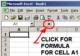
2. The FORMULA Bar then appears.
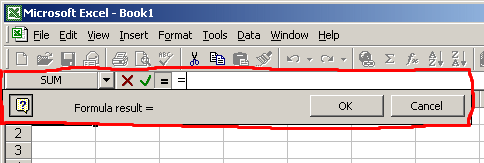
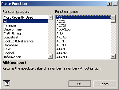
3. In order to see all the available formulae, click on the Drop-Down menu: and at the bottom of the list/ menu select 'More Functions...' to bring up the
following dialog box:
4. Create the following Table and using the appropriate FORMULA (Sin, IF,
Cos, etc) calculate the unknown (?) values.
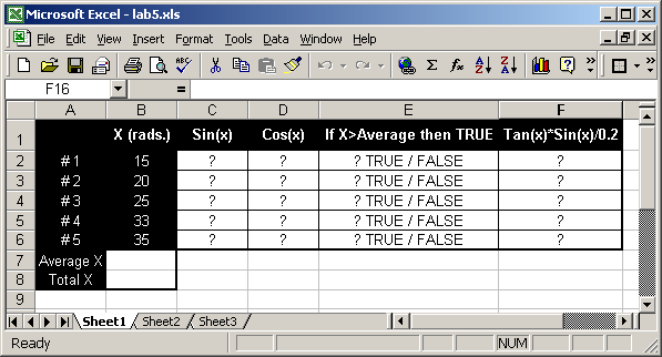
Make sure to use IF statements/ formulae to show whether X is greater than the
Average X, by Means of a True/ False answer.
5. Use Conditional Formatting to automatically apply Green Shading to cells
answering "TRUE" and Red Shading to cells answering "FALSE".
How To: Highlight all the cells you wish to apply
conditional formatting to. Then from the FORMAT Drop-Down menu, select
"Conditional Formatting". Select an appropriate "Condition"
that will recognise when the value in a cell is TRUE or FALSE. Two separate
Conditions will have to be used.
Click Here for Solution, if all else fails ->>
Exercise 2: (Graphs in
Excel)
1. Open the Microsoft Excel Application, and create the following spreadsheet
for the gas and electricity costs as shown below:
| |
1989 |
1990 |
1991 |
1992 |
| Electricity |
12 |
15 |
18 |
22 |
| Gas |
6 |
8 |
15 |
17 |
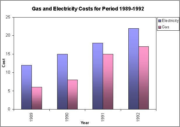
2. Using the Chart Wizard  , create the graphical representation of the data as
shown below:

Hints: All of the options chosen in the Chart Wizard, can
be changed afterwards, by Right-Clicking on any part of the chart.
In order to change the Alignment of the years text, Right-Click on the years,
and go to "FORMAT AXIS"
Further Help Available on making the graph HERE>>
3. Use a second WorkSheet within the same Excel Spreadsheet, and create the
following table of information showing the resistance of Inks with varying
heights of print.
|
Ink A |
Ink B |
Ink C |
Ink D |
Ink E |
| 13 micrometers |
939.00 |
900.64 |
1329.43 |
38.36 |
1.25 |
| 40 micrometers |
381.01 |
462.07 |
526.29 |
17.57 |
0.70 |
| 80 micrometers |
342.36 |
368.74 |
364.84 |
7.69 |
0.60 |
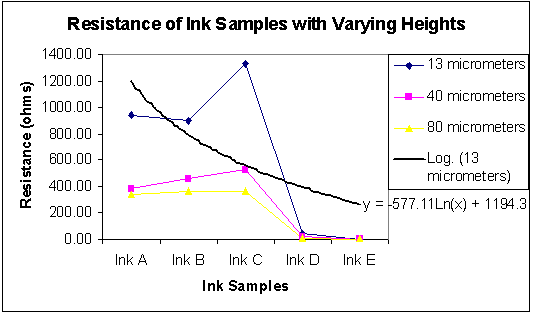
3. Using the Chart Wizard  , create the graphical representation of the data as
shown below:

4. Add a Trendline and an Equation for one of the Heights (13, 40 or 80
micrometers)
Hints: Use a Line Type Graph, with markers shown at each data value.
A Trendline MUST BE added firstly, before attempting to add an equation.
How to add an Equation: RIGHT-CLICK on the TRENDLINE and in the options tab,
select "Show Equation on Chart"
Exercise 3: (Sorting Data and Printing in Excel)
1. Map the following Network Drive: \\europa\ie4711
2. Inside the Lab_5 folder, open the lab_5.xls file. Click "Save As"
from the FILE Drop-Down menu and save to your WorkArea.
3. In Column C, use the "CONCANATE" formula to complete the ID Number
for the 150 students.
4. In Column E, use the "PROPER" formula to Tidy/ remove Capitals from
the first name.
5. In Column G, use the "LEFT" formula to select only the first
Initial of the First names.
6. For Column H, use the appropriate formulae to give the required result as can
be seen in the Light-Green Shaded Cells.
7. Use the SORT facility in Excel, to Sort all the data, based on the First Name
of Students, to arrange the data in alphabetical order.
Hint: Select all the data to be sorted (Columns and Rows
complete), from the DATA Drop-Down menu select SORT. Sort based on the First
Name.
8. Select Print Preview to see how Excel would print the document. (From
the FILE Drop-Down menu, select "Print Preview")
9. Notice how Excel will take 12 pages to print the document, many of which have
little or no data.
10. Close the Print Preview (Press Esc, Top left of Keyboard).
11. Go to the Print Setup of the document. (From the FILE Drop-Down menu, select
"Page Setup")
12. In the page tab, select LANDSCAPE, and choose to "FIT to 1 page wide by
2 tall.
13. Go back to Print Preview and preview the changes.
14. The Margins can be changed to increase the printable area. (Click on the
'Margins' in the Print Preview. Click and drag the back ticks |
)
15. Click "Page Break Preview" to view and adjust the amount of data
per page. To exit, go to the VIEW Drop-Down menu and select "Normal"
View.
16. See if the Titles: [Short ID No] [Full ID No] [Surname] [Remove Capitals of Surname]
[First Name] [First Initial of First Name] [First Initial] [Surname] [Full Course]
can be printed on the top of every page printed out in Excel.


 and at the bottom of the list/ menu select 'More Functions...' to bring up the
following dialog box:
 , create the graphical representation of the data as
shown below: